What to Expect When You're Expecting Value

How should you incorporate explicit expected value estimates into your prior beliefs? Some help from the Kalman filter

NB: This post, first, largely recapitulates a series of several long posts from the early 2010s GiveWell Blog. I’m aiming to explain these ideas in a much shorter, more intuitive way. Then, I discuss some further implications for approaching integrating explicit estimates into one’s all-things-considered reasoning.

Suppose you’ve done some analysis or made some estimate of the likely impact of an action — say, the expected ethical value of a career in artificial intelligence (AI) safety, or the dollar-equivalent value of a career in global health and development, or the value of growing effective altruism. And, further, you’ve done a pretty exhaustive job! You’ve included all the possible effects you can think of, even when they’re hard to have a stable view on, and put a probability and value on each consideration. You’ve even used probability distributions to quantify your uncertainty with, when you’re really unsure, extremely wide error bars. This explicit model spits out some result in terms of expected reduction in risks from advanced AI, or lives saved, or careers influenced.

Should you, having made this estimate, adopt the average value of the resulting probability distribution as your best guess, even when the resulting distribution is extremely uncertain? In other words: you’ve done your best, included everything you can think of in your explicit estimate, and come away thinking that the resulting expected value is as likely to be too high as too low. Do you take it literally?

There’s a temptation to say, “Well, this is my best guess — if there were more factors I thought were relevant, then I would have included them in the model!”

This, I think, would be a mistake. The key takeaway from what follows is that, the more uncertainty exists in the model, the less weight one should give the results. In some sense, this is intuitive — if the results are extremely sensitive to some factor where you’re hugely uncertain and could easily be off by a factor of something like a thousand or a million, then it seems obvious that you should treat that differently than a sure bet with equivalent expected value.¹ But, if both estimates have the same expected value, it seems hard to justify this in a more rigorous way. What’s going on here?

What I am and am not saying

I’m not saying that quantitative estimates are useless for decision-making.

• I am saying that the point-estimate of e.g. expected value, often reported as the headline figure from a quantitative estimate of the kind described above, is often pretty unhelpful when the uncertainty of the estimate is large.

• Quantitative modeling can also be helpful for deciding what to research more. If your estimate has enormous uncertainty coming from a few key sources, getting more information to reduce those uncertainties can be really valuable.

I’m not saying that one should avoid making bets on low probabilities with high payoffs, like running for political office or working to prevent extreme tail risks from worst-case climate change scenarios.

• There’s some nuance here about the structure of uncertainties. If we know the probabilities of extreme climate change scenarios in the next 100 years is around 2%, give or take 2%, then the probabilities are low but robust (Case 1). If, on the other hand, we could only say that the probability of extreme climate change scenarios was somewhere from 0.000001% to 50%, then the uncertainty bounds on our model would be very large (Case 2).

• I am saying that we should move less from our prior beliefs when we have larger uncertainty in the estimate, as in Case 2 above. Another way of putting this is that when a model’s ultimate expected value is highly sensitive to very uncertain parameter estimates, we should trust it less.

With that out of the way: Ok, so how should I interpret an explicit estimate, ranging from a quick back-of-the-envelope estimate to a more serious probabilistic model to compare two high-impact interventions?

A Quick Detour Into Control Theory

In the process of researching this question, I bumped into an analogy from engineering (more narrowly, control theory) that I find helpful here. I’ll use the standard example in the introductions I read: tracking the position of a car. (This is an extremely simplified explanation that aims to do just enough to make the analogy work. I’m not an engineer!)

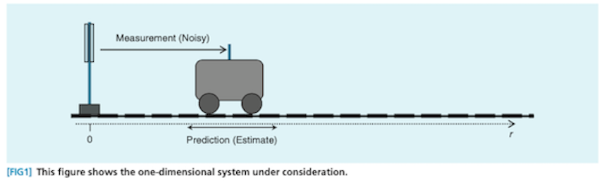
So, suppose you have a car that’s driving and you want to keep track of its position. You have two sources of information: the velocity of the car (speed and direction) and a GPS monitor. Since you know the velocity is, say, 88 feet per second (or 60 miles per hour) heading north, you might predict that the car will be 88 feet further north in one second. We can’t be sure though, since the car might accelerate or decelerate, or be buffeted by wind, or something else! Our prediction might therefore center on 88 feet north, but with some error bars in either direction.

That’s step one: make a prediction. The next step is taking a measurement of the car’s position using the GPS monitor. Unfortunately, our GPS doesn’t have great signal. That means we again get a prediction of the position, but again with some error bars in either direction. So, how do we combine these two estimates?

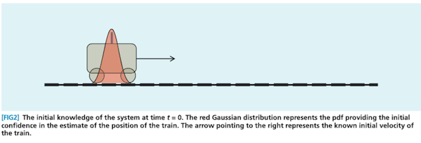
Here’s what that might look like if, instead of a car, you had a cute little train and slightly different prediction and measurement sources: ²

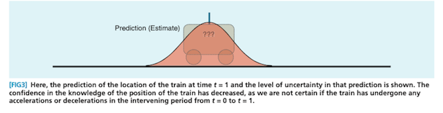
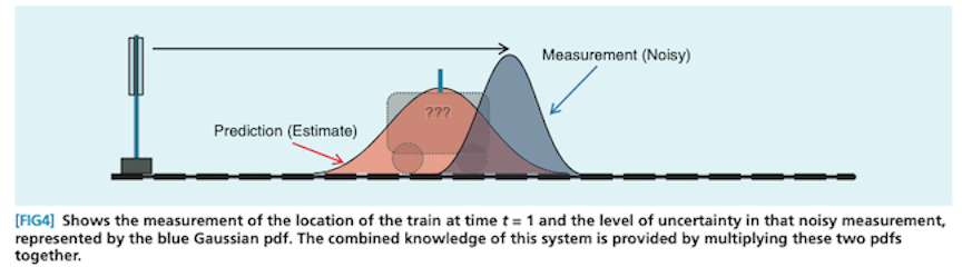
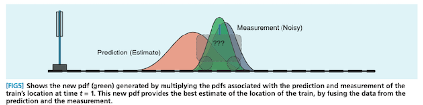
Notice that the prediction distribution is significantly more uncertain (and hence wider) than the measurement distribution. Consequently, the all-things-considered estimate ends up closer to the measurement than the prediction. This is an important behavior: when your prediction is more uncertain relative to the measurement, you should move more in the direction of the estimate. The reverse is also true.

This algorithm, where you predict, measure, combine, and repeat, is called the Kalman filter. The standard Kalman filter is the optimal way to estimate the state of one-dimensional linear systems so long as both the prediction and measurement errors are independent and normally distributed (the bell-shaped curve).³ Somewhat intuitively, the best estimate of position we can make is one that maximizes the probability of both the prediction and the measurement being correct.⁴ This is done by multiplying the two distributions together, which in this case yields (after re-scaling) another Normal distribution.⁵

The Kalman filter is particularly convenient because the resulting estimate is a Normal distribution, which then constitutes the jumping-off point for another cycle of prediction, measurement, and combination, all the while maintaining its small computational requirements. Moreover, additional noisy estimates can be incorporated in the same way, by recursively updating based on the new measurements.

Back to Business

You’re interested in the expected impact of, say, working to reduce the risk of nuclear conflict as a career diplomat. You have some prior belief about how the expected values for careers in public service are distributed, and you’ve done an explicit estimate of the expected impact of you trying to make it to the upper echelons of US nuclear weapons policymaking. How does the Kalman filter analogy help?

Because you’re trying to estimate the expected impact of this career path, that’s the thing you’re trying to measure: the state of interest. It’s analogous to the position of the car above. Your prior belief is the prediction, analogous to predicting the position using the known velocity. The explicit expected impact estimate is the measurement, analogous to the GPS signal. And, finally, the combined all-things-considered estimate of the expected impact is arrived at the same way as the combined estimate for position.

As before, when your prior belief (“prediction”) is more uncertain relative to the explicit estimate (“measurement”), you should move more in the direction of the explicit estimate (“measurement”), and vice versa.

Just how much does the uncertainty matter, relative to the mean? It appears to matter a whole lot. Here’s a chart I made displaying the phenomenon when your prior belief is described by a standard Normal distribution (i.e. a Normal distribution with zero-mean and a standard deviation of one) and your explicit estimate is also a Normal distribution, with some mean and some standard deviation.⁶

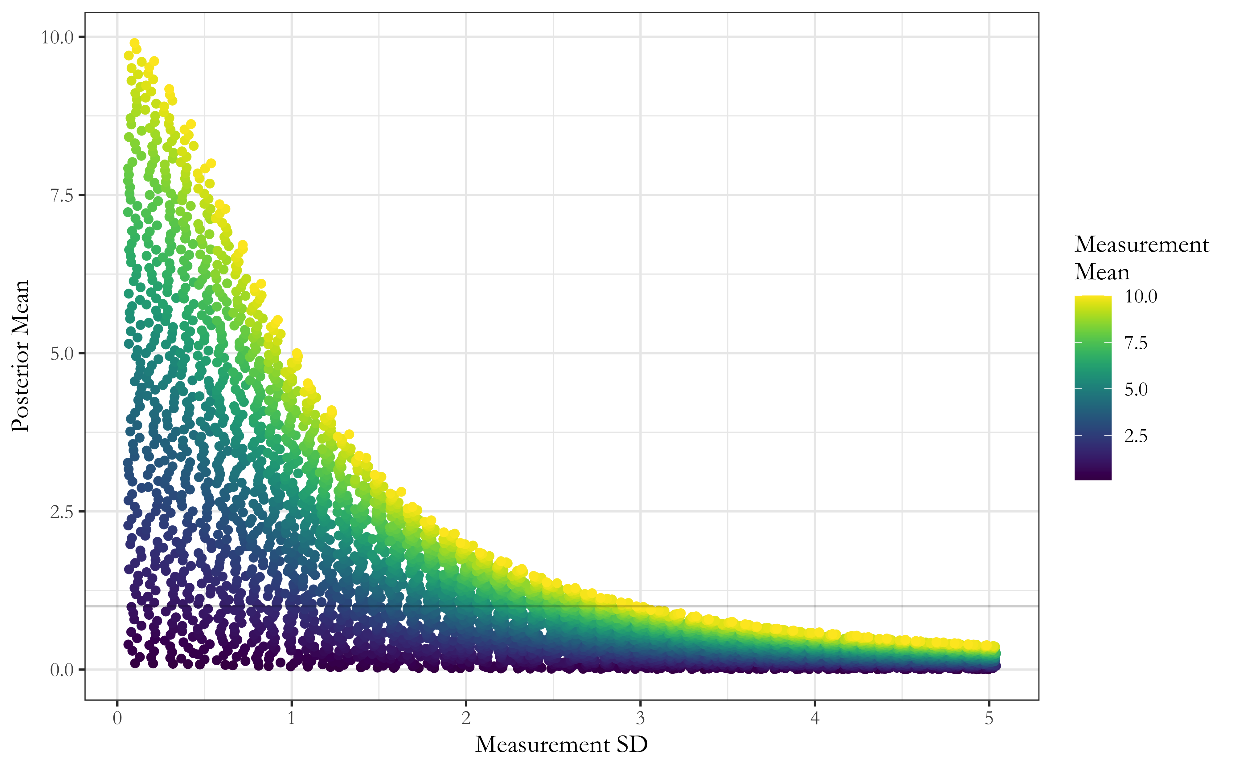
Here’s the headline result: as the uncertainty in your estimate for expected impact grows, the estimate’s influence on your ultimate conclusion should rapidly diminish. On the other hand, estimates with extremely narrow uncertainty bounds should move you very substantially in their direction.

On the vertical axis, you have the posterior mean. This is the all-things-considered mean value you end up with once you’ve combined your prior beliefs with your estimate, and it represents your (standardized) best guess at the true value you’re trying to estimate (here, the expected impact of a career diplomat). Larger numbers represent more impact.

On the horizontal axis, you have the measurement standard deviation. This represents the uncertainty associated with your estimate. Larger numbers represent more uncertainty. Finally, the data points are colored by the measurement mean, which is the best guess that your estimate spits out. As before, larger numbers represent more impact.

When the estimate is highly certain and hence has a standard deviation near 0, notice that the measurement mean and the posterior mean are nearly equivalent. (Look at the data points adjacent to the vertical axis to see this.)

You can think of our all-things-considered best guess (“posterior mean”) as a function of the uncertainty in our estimate (“measurement standard deviation”). I’m following standard statistical graphics norms here, where the explanatory variable is plotted on the horizontal axis and the response variable is plotted on the vertical axis.

Here’s what this looks like in individual cases:⁷

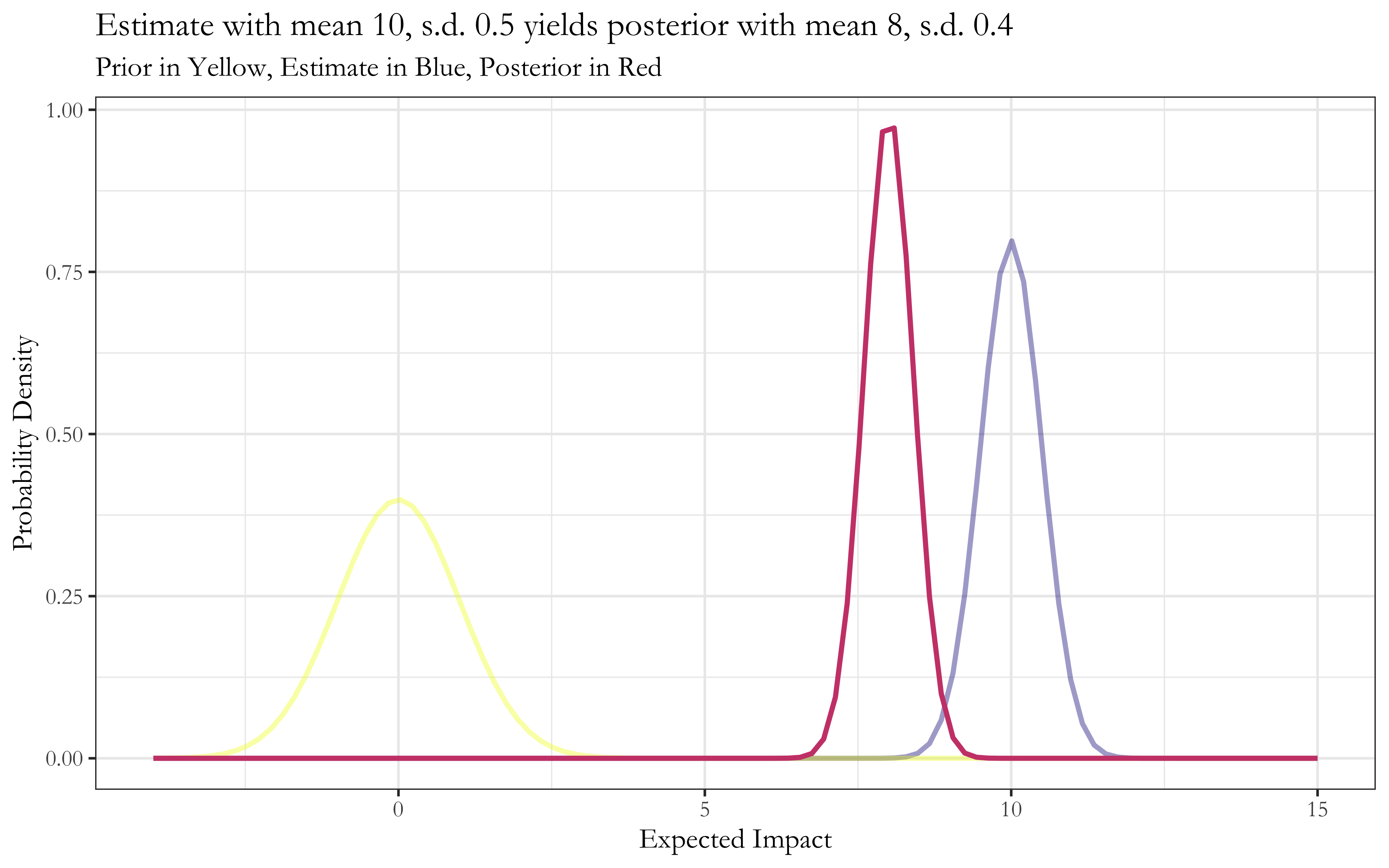
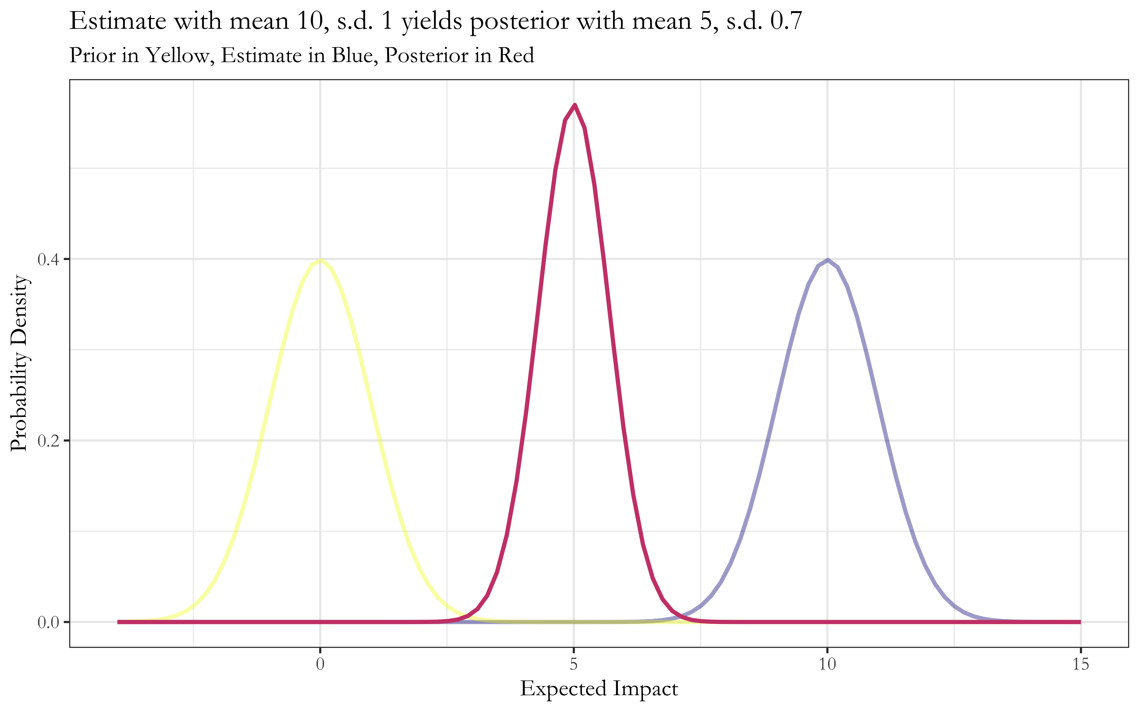
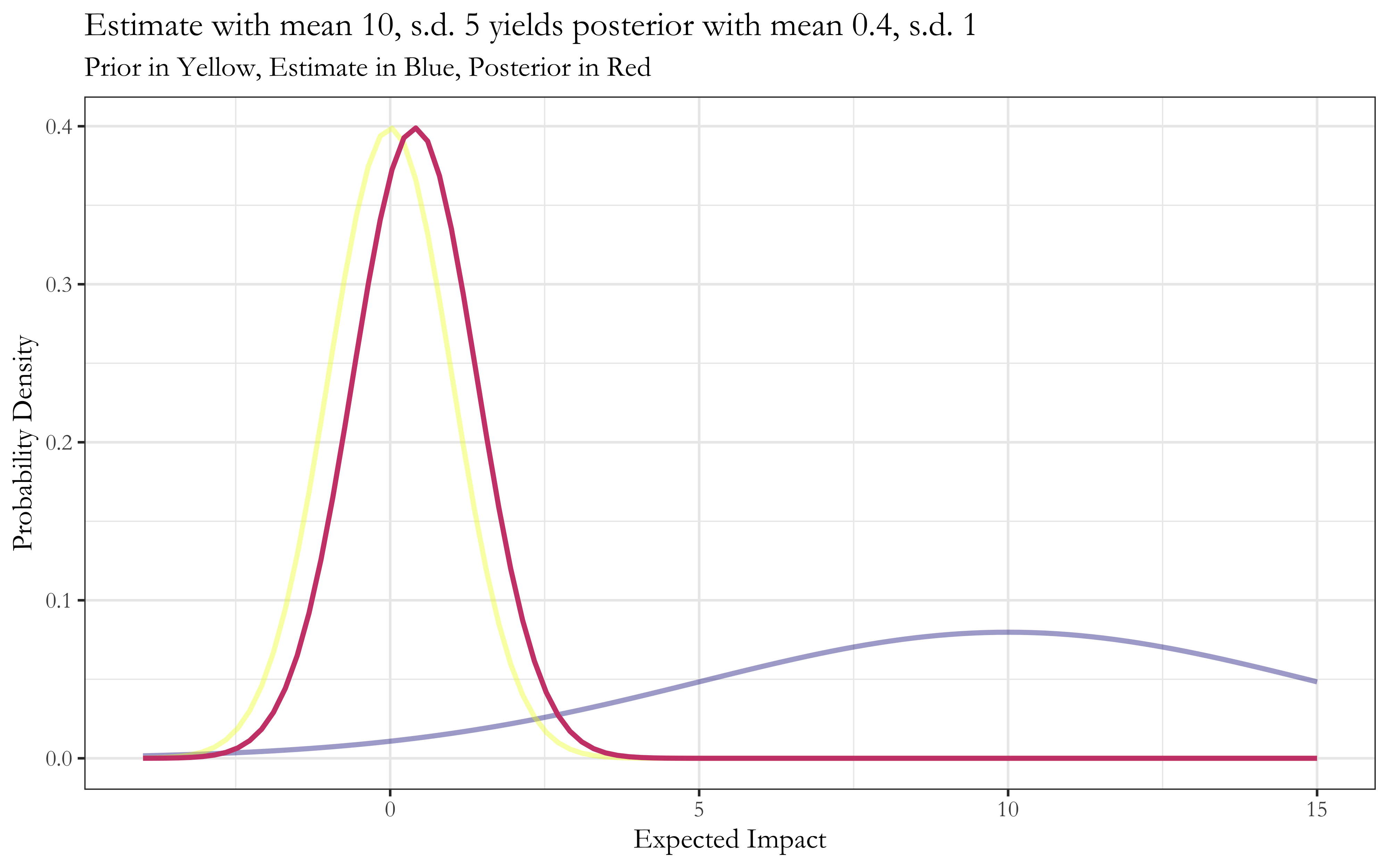
Now, this setup was chosen due to its nice features and computational simplicity. The results are therefore fairly specific to the Normal distribution and its previously noted elegant property wherein the renormalized product of Normal distributions is again a Normal distribution. Nonetheless, the broad conceptual implication holds when our beliefs and estimates take the form of log-normal distributions, which share the same multiplicative property.

And because many situations (arguably including impact) are multiplicative processes that can be modeled as log-normal distributions, there’s reason to think that these broad conceptual implications apply in many relevant cases.

Right now, I’m not sure how this generalizes to other scenarios where, for instance one’s prior belief is log-normally distributed and one’s estimate is shaped like a power law distribution. Moreover, one can only straightforwardly multiply distributions in this way if the two distributions are statistically independent, which is rarely the case. Is there a simple way to combine distributions in those cases without tons of math? I hope to explore the implications of these cases and more in future work.

Endnotes